Extended Kalman Filter SLAM
SLAM, EKF, C++, ROS2, Open Robotics Turtlebot3 Burger, 2D LiDar
Description
In this project, I designed and implemented a Simultaneous Localization and Mapping (SLAM) algorithm based on the Extended Kalman Filter (EKF) over the ROS2 platform from scratch for a Turtlebot3 Burger. This system enables the robot to simultaneously build a map of its environment while localizing itself within that map, using only wheel odometry and 2D LiDAR sensor data.
System Overview
graph TB
    subgraph Sensors["Sensor Input"]
        LIDAR[2D LiDAR Scanner]
        ENCODERS[Wheel Encoders]
    end

    subgraph Processing["SLAM Processing"]
        ODOM[Odometry Model<br/>Forward Kinematics]
        CIRCLE[Circle Detection<br/>Clustering & Fitting]
        EKF[Extended Kalman Filter<br/>State Estimation]
        ASSOC[Data Association<br/>Landmark Matching]
    end

    subgraph Output["State Estimation"]
        POSE[Robot Pose<br/>x, y, θ]
        MAP[Landmark Map<br/>Obstacle Positions]
    end

    ENCODERS --> ODOM
    LIDAR --> CIRCLE
    ODOM --> EKF
    CIRCLE --> ASSOC
    ASSOC --> EKF
    EKF --> POSE
    EKF --> MAP

    style LIDAR fill:#e1f5ff
    style EKF fill:#fff4e1
    style POSE fill:#d4edda
    style MAP fill:#d4edda
Demo Video
This project consists of two main tasks, which are:
SLAMwith known associationSLAMwith unknown association
SLAM with known data association
SLAM with unknown data association
Software Structure
The overall structure of the project is shown in the flowchart below:
flowchart TD
    START([Initialize System]) --> ODOM_INIT[Initialize Odometry<br/>Wheel Encoders]
    ODOM_INIT --> SLAM_INIT[Initialize EKF SLAM<br/>State Vector & Covariance]

    SLAM_INIT --> SENSE[Sensor Update Loop]

    SENSE --> READ_ENC[Read Wheel Encoders]
    READ_ENC --> PREDICT[EKF Prediction Step<br/>Update Robot Pose]

    PREDICT --> READ_LIDAR[Read LiDAR Scan]
    READ_LIDAR --> CLUSTER[Cluster Point Cloud<br/>Unsupervised Learning]

    CLUSTER --> FIT[Fit Circles to Clusters<br/>Extract Landmarks]

    FIT --> KNOWN{Data Association<br/>Mode?}

    KNOWN -->|Known| MATCH_KNOWN[Use Known IDs]
    KNOWN -->|Unknown| MATCH_UNKNOWN[Mahalanobis Distance<br/>Matching Algorithm]

    MATCH_KNOWN --> UPDATE[EKF Update Step<br/>Correct with Landmarks]
    MATCH_UNKNOWN --> UPDATE

    UPDATE --> PUBLISH[Publish Corrected Pose<br/>and Map]
    PUBLISH --> SENSE

    style START fill:#d4edda
    style PREDICT fill:#fff4e1
    style UPDATE fill:#e1f5ff
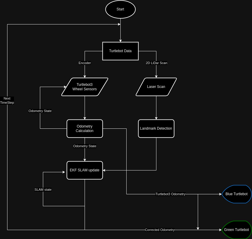
Original system structure diagram:
Odometry Model
To get the odometry from the wheel angle and velocity, it applied kinematics model from Modern Robotics to conduct the Forward Kinematics and Inverse Kinematics of the robot.
The geometry model of the robot can be present using \(H\) matrix.
\[\begin{align*} H(\theta) &= \begin{bmatrix} h_1(\theta) \\ h_2(\theta) \end{bmatrix} \\ h_i(\theta) &= \frac{1}{r_i \cos{\gamma_i}} \begin{bmatrix} x_i \sin{\left (\beta_i + \gamma_i \right )} - y_i \cos{\left (\beta_i + \gamma_i \right)} \\ \cos{\left ( \beta_i + \gamma_i + \theta \right )} \\ \sin{\left ( \beta_i + \gamma_i + \theta \right )} \end{bmatrix}^\intercal \end{align*}\]For the Turtlebot3, which is a diff-drive mobile robot. The parameters are defined as
So that \(H(0)\) can be calculated as
\[H(0)=\begin{bmatrix} -d & 1 & -\infty \\ d & 1 & -\infty \end{bmatrix}\]Where \(d\) is the one-half of the distance between the wheels and the \(r\) is the radius of the wheel.
Hence \(F\) matrix can be calculated by
\[F=H(0)^\dagger = r \begin{bmatrix} -\frac{1}{2d} & \frac{1}{2d} \\ \frac{1}{2} & \frac{1}{2} \\ 0 & 0 \end{bmatrix}\]Forward Kinematics
The forward kinematics is to find the tranform from current state to next state \(T_{bb'}\) given the change in wheel positions \(\left( \Delta\phi_l, \Delta\phi_r\right)\).
- Find the body twist \({\cal V}_b\) from the body frame of the current state to next state:
- Construct the 3d twist by
- Then, the transform from current state to next state \(T_{bb'}\) can be calculated by
Inverse Kinematics
Inverse kinematics is to find the wheel velocities \(\left(\dot{\phi_l}, \dot{\phi_r} \right)\) given the body twist \({\cal V}_b\).
The wheel velocities can be calculated as
\[\begin{bmatrix} \dot{\phi}_l \\ \dot{\phi}_r \end{bmatrix} = H(0){\cal V}_b = \frac{1}{r}\begin{bmatrix} -d & 1 & -\infty \\ d & 1 & -\infty \end{bmatrix} \begin{bmatrix} \omega_z \\ v_x \\ v_y \end{bmatrix}\]Since this robot is non-holonomic so that it cannot move sideways. Hence \(v_y=0\), then the wheel velocities \(\left(\dot{\phi_l}, \dot{\phi_r} \right)\) are:
\[\begin{align*} \dot{\phi}_l &= \frac{1}{r} \left ( -d \omega_z + v_x\right) \\ \dot{\phi}_r &= \frac{1}{r} \left ( d \omega_z + v_x\right) \\ \end{align*}\]SLAM Algorithms
There are two key algorithms implemented in this project: the Extended Kalman Filter (EKF) for state estimation and the Circle Fitting Algorithm for landmark detection.
graph LR
    subgraph EKF["Extended Kalman Filter"]
        PRED[Prediction Step<br/>Motion Model]
        UPDATE[Update Step<br/>Measurement Model]
    end

    subgraph Detection["Landmark Detection"]
        CLUSTER[Data Clustering<br/>Unsupervised Learning]
        FIT[Circle Fitting<br/>Least Squares]
        ASSOC[Data Association<br/>Mahalanobis Distance]
    end

    PRED -->|Predicted State| UPDATE
    CLUSTER --> FIT
    FIT --> ASSOC
    ASSOC -->|Landmark Observations| UPDATE
    UPDATE -->|Corrected State| PRED

    style PRED fill:#fff4e1
    style UPDATE fill:#e1f5ff
    style CLUSTER fill:#d4edda
Extended Kalman Filter (EKF)
The EKF algorithm enables the robot to localize itself using the positions of all detected landmarks relative to its current pose. The algorithm operates through conditional probability:
sequenceDiagram
    participant State as Robot State (x,y,θ)
    participant Motion as Motion Model
    participant Sensor as Sensor Model
    participant Landmarks as Landmark Map

    Note over State: Time step k

    State->>Motion: Apply control input (wheel velocities)
    Motion->>State: Predict new pose (x',y',θ')
    Note over State: Prediction increases uncertainty

    Sensor->>Landmarks: Detect landmark positions
    Landmarks->>State: Compare predicted vs observed
    Note over State: Innovation (measurement residual)

    State->>State: Compute Kalman Gain
    State->>State: Correct pose estimate
    Note over State: Reduced uncertainty

    Note over State: Updated state at k+1
Key Steps:
- Prediction: Use odometry to predict the robot’s next state based on wheel velocities
- Innovation: Compare predicted landmark positions with actual observations from LiDAR
- Correction: Compute the weighted correction using Kalman gain
- Update: Adjust both robot pose and landmark positions to minimize uncertainty
Circle Detection
Data Clustering
This component employs Unsupervised Learning (clustering algorithm) to group LiDAR point cloud data, identifying which points belong to the same cylindrical landmark.
Circle Fitting
Using Least Squares optimization, the algorithm fits circle parameters (center position and radius) to each cluster of points, extracting precise landmark locations.
Data Association
Data association determines which detected circle corresponds to which previously observed landmark:
- Known Association Mode: Landmark IDs are pre-assigned
- Unknown Association Mode: Uses Mahalanobis distance to match observations with the landmark map, handling new landmark initialization when needed
Packages
nuturtle_description: Visualizing the pose of the turtlebot3 burgerturtlelib: Call customized library functions for kinematics and slam calculations.nusim: Simulate the turtlebot in the real world.nuturtle_control: Performing the turtlebot kinematics calculation and parsing the command sent to theturtlebot3.nuslam: Performs the SLAM algorithm for correcting the error odometry.